
Excel’s Indirect function allows the creation of a formula by referring to the contents of a cell, rather than the cell reference itself. Of all the functions covered in our Excel courses, it is often Indirect() that attendees haven’t come across but find an immediate use for, often saving a great deal of time and effort in the process.
If you have several sheets, each with information for a single department for example, you may want to set up a summary sheet. Rather than creating separate formulae to refer to each sheet, Indirect() can allow you to create a single set of formulae all of which use a reference to a sheet name held in a cell – hopefully an example will make this clearer.
To refer to cell A2 on a sheet named ‘Cuddly Toys’ we would use a formula like this:
=’Cuddly toys’!A2
However, sometimes it would be useful to be able to change a whole series of references to, for example, a different sheet.
We could type the sheet name into a cell on our main sheet, say A1. We could then write a formula to refer to cell A2 on the sheet typed into cell A1.
If we simply type:
=A1!A2
Excel, not unreasonably, looks for a sheet named A1 and fails to find it.
However, we can use the Indirect function instead. Here is the screen from the Paste Function dialog for Indirect:

“‘“ & $A$1 & “‘!A2“
Our Ref_text entry is a little confusing, so we have highlighted the pairs of speech marks in different colours. We have two items of text, and sandwiched in between them, an absolute reference to the contents of cell A1 – as you can see this correctly returns the contents of that cell – Cuddly toys. The ampersands are used to join the 3 elements of our Ref_Text together. The first text section simply holds a single apostrophe – this is necessary because, if our sheet name contains a space, it must be surrounded by apostrophes to be correctly identified. The second section contains an absolute reference to cell A1 – the cell where we type the name of our sheet. The third text section contains the closing apostrophe for the sheet name, together with the exclamation mark that separates sheet name from cell reference, and the cell reference itself – A2.
This works well to return the contents of cell A2 on our cuddly toys sheet, and if we were to type in ‘Boardgames’ for example, it would automatically return the contents of cell A2 on a sheet named ‘Boardgames’.
However we do have a problem left to solve. We need to refer to many cells on the price list sheets, but if we copy our Indirect cell, the reference to A2 doesn’t change, because it is just text. We can solve this by using a row/column style reference instead of A2:
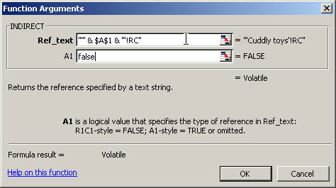
“‘“ & $A$1 & “‘!RC“
Note that we have to set the ‘A1’ argument of the function to ‘False’ to use this reference. RC will return the current row and column – so a formula in cell A2 will refer to A2 on cuddly toys, A3 to A3 and so on. If we need to refer to a different cell we would add numbers in square brackets after R and C. So R[1]C[1] would look at the cell one row down and one column right for example.


Superb!!
Greetings. I have been using INDIRECT for some time and find it very useful. However, I can’t seem to figure out a way to use it to reference a range across several worksheets. I can get the range working okay on one worksheet, but not several. There is no indication that you can’t do this, so I am still trying. Any suggestions? This would allow me to pick up YTD figures from a series of identical mthly worksheets with just one cell change – if I can get it working.
Hi Doug
Good question and one that doesn’t seem to have an easy answer. There is a discussion and rather involved possible answer here:
http://www.eggheadcafe.com/software/aspnet/31803284/how-do-i-set-up-a-3d-refe.aspx
Hey there,
Can you help me with my query, i have several worksheets in one workbook containing different expenses, what i am looking for is to make a summary page in which the expense total of each entity from different work sheet comes up automatically every times its get changed.
Rgds,
Amm.
Hi Amran
If I understand correctly, it depends on whether you can include a cell on each worksheet that calculates the sum of the expenses you want. If so, you could give each of the cells in the individual worksheets a different name (in case their position changes) then refer from the summary worksheet with something like: =Asheet!Asum, =Bsheet!Bsum etc. If the individual summaries cells are static you could just link to the cell reference e.g. =Asheet!C1 or whatever.
Can you tell me how to propery delimited this formula?
=SUM(IF(indirect(C1)!$E$2:$E$500=”N”,1,0))
No matter what combination of quotes I try I keep getting an error…
C1 = May08 (sheet name)
Thanks!
James
Hi James
There are a few problems with what you have at the moment, in particular the E2:E500 bit. If what you are trying to do is to count the cells in the range that contain the letter N (lower or upper), try something along the lines of (do check carefully – no guarantees!):
=COUNTIF(INDIRECT(C1 & “!$E$2:$E$500″),”N”)
Let me know if this is what you want.
Kind regards
Simon
Let
Fantastic!
I just found the indirect function, but wanted to know how to update the references, and yours helped.
My case is i have two lists of ordered numbers but not all numbers are in both lists. For a quick comparison, i use (in column C) =A1=B1 (and conditional formatting to turn FALSE into read, and !FALSE to green), and drag the field to populate all the fields in column C.
The problem is that when i find a gap, i either add empty fields, or cut & paste the fields to match the other column (leaving the gap there). The purpose, is so all populated fields match.
The problem was that cut&paste or adding that field, updated the reference. Hence indirect, but then indirect could not be easily automagically copied.
Using this post helped. I could not quite figure our how to use your final example, but i did finally get it with =INDIRECT(“R” & ROW() & “C1”, FALSE) = INDIRECT(“R” & ROW() & “C2”, FALSE).
Thanx for the post.
Hi Brian – thanks very much for your comment – glad the post helped, and well done on working out how to adapt it to solve your problem.
Regards
Simon
I’m successfully able to create data using indirect statements, to result in for example “John Smith”. However, I’m trying to use this as the reference for a vlookup on other data. It’s not working. What I’m finding is that I also cannot perform a simple “find” on the generated data using Ctrl-F and entering “John”, which is probably a precursor to using this as a reference in a VLookup statement. Any ideas how to make the resultant Indirect information recognizable?
Thank you.
Hi Scott
The find should work if you set the find options to search values rather than formulas, and indirect() should work OK as the lookup value in a Vlookup function. I’ve tried it on a simple example without a problem – could you give me a bit more information about the Indirect and Vlookup formulae you are using?
Regards
Simon
It turns out that my spreadsheet was large and it was taking several minutes to calculate. I wasn’t waiting those several minutes. Everything is working now.
Thanks, Scott
Thanks for the help with the Indirect function. Here is my problem.
When I use =INDIRECT(A1) in SheetA where A1 points to cell D1, I get the value of D1.
However, I need to reference cell A1, as above, from SheetB. The formula I am using is =INDIRECT(Sheet1!A1)
This returns the value 0 and not the value of D1 in SheetA
Any help would be appreciated.
Guy
Thanks Guy – did you mean:
=INDIRECT(“SheetA!A1”) ?
Presumably there’s some good reason why you’re using INDIRECT() rather than just the formula =SheetA!A1?
Regards
Simon
I’m adding in one row each day to SheetA, at row 1 so that the info in D1 today, becomes D2 tomorrow. However, I don’t want the reference to refer to D2, tomorrow, but to D1.
Regards,
Guy
Thanks Guy – I understand now – did you get it to work with the SheetA reference in the end?
Regards
Simon
Yes, I did get it to work. Here’s the principle.
I have two worksheets, Sheet1 and Sheet2. Column D, (D1,D2,D3, etc.), in Sheet1 needs to call the data from Column A, (A1, A2, A3, etc.), in Sheet2.
However, since I am adding rows above row 1 in Sheet2 on a daily basis, I still want D1 in Sheet1 to call from A1 in Sheet2. The problem is that if I want to add a row to Sheet2, all of my references increment by 1 in Sheet1 so that D1 in Sheet1 points to A2 in Sheet2 and not to A1.
Solution:
I added the following to column A in Sheet1:
Cell A1: Sheet2!A1
CellA2: Sheet2!A2
CellA3: Sheet2!A3
Etc.
Note: There is no “=” sign before the entry.
Now I pointed D1 on Sheet1 to A1 on sheet1 using the indirect function shown below. Since A1 is text and not a formula, no “=” sign, it does not increment when I add a row to Sheet2, which means that it will always point to the same absolute reference.
Therefore; Cell D1 in Sheet1, calls the info from Cell A1 in Sheet1, which in turn calls the information from Cell A1 in Sheet2.
The formula for D1 on Sheet1 looks like this:
=INDIRECT(A1)
as opposed to
=INDIRECT(Sheet2!A1) which returns a #REF.
Hope that helps.
Guy
Hi Guy
I’m not sure whether you just didn’t put the quotes in the comments, or they didn’t come through on the blog, but I think =INDIRECT(Sheet2!A1) should be =INDIRECT(“Sheet2!A1”)
I think that should avoid the need to enter the text in column A. I hope I’ve understood correctly this time.
Regards
Simon
Thanks. That’s even better.
Simple, when you know how.
🙂
Guy
I have been using the Indirect function for quite sometime. But I have always used it to refer to values on some other worksheet of same workbook as you have shown in your example.
can we use it to refer to value of cell in another work book save some where without opening it (like we use links) this will help us to change the path of the file in one cell and hence the values. I am trying for the same but its not working and always gives me #REF ! error. Any help available on this issue.
Hi Anupam – I’m pretty sure that you will always get #REF when using INDIRECT() with a closed workbook. The Contextures site has a detailed description of the use of INDIRECT() including reference to its inability to cope with closed workbooks:
http://www.contextures.com/xlFunctions05.html
Hi Guys,
I was wondering if you could help me please, I am new to Excel,
I need to use (add) indirect function to the following formula:
=IF(‘Time Sheet Entry’!A14=””,””,CONCATENATE(“|”,FIXED(‘Time Sheet Entry’!S14,2),”|”))
Can someone help me with this please?
thanks
If you just want to replace the sheet name entry using Indirect() then the following should cope – it uses whatever is entered into cell A1 as the sheet name, or were you after something different?
=IF(INDIRECT(“‘”& A1 & “‘!A14″)=””,””,CONCATENATE(“|”,FIXED(INDIRECT(“‘”& A1 & “‘!s14″),2),”|”))
Hi Simon
thanks for your reply,
What i AM trying to do is in SHEET2 i am using the above forumla to refer to sheet1 but whenever I delete the row in sheet1 , the forumla returns #REF which is fine beacuse the row is been delete but the row is now replaced with the new 1, why does it still return #ref? as I have a new valuse:
e.g.
a b
1 5 5
2 6 6
3 7 7
if I now delete the row 2, row 3 replaces row 2 but in sheet2 , the forumal still return #ref , instead of haveing the new value say 7,
could please help? I have looked and some people say there diffrent type of referencing and that you could use maybe undirect,? is that rigth?
thanks
Hi
I think what they are referring to is the use of INDIRECT() to ‘fix’ a cell reference so that reference always refers to what is currently in that cell, unadjusted for insertions and deletions. For example the following ‘Row/Column’ form of an INDIRECT() function (note the extra argument of ‘False’ at the end to use Row/Column rather than A1 referencing) would always refer to the same cell in the sheet named in cell $A$1 as the cell that contains the formula. RC meaning no rows, no columns offset from the current location – if it was typed into cell D14 it would refer to D14. R[1]C[1] would refer to E15 etc.)
=INDIRECT(“‘”&$A$1 & “‘!RC”,FALSE)
hi simon
that’s exaclty what i am trying to do but how do i use it or include it within the following formula, beause everytime i am trying to add indirect , my forumla return syntzt errorr
=IF(‘Time Sheet Entry’!A14=””,””,CONCATENATE(“|”,FIXED(‘Time Sheet Entry’!S14,2),”|”))
even tho I am java developer to be honest i am stuck with this, could you pleaseee, see if you can solve this?
Try this – do test carefully. Again assumes sheet name is in A1. Also assumes formula is entered in A14, hence the second reference is offset by 18 columns from A to S:
=IF(INDIRECT(“‘”& A1 & “‘!RC”,FALSE)=””,””,CONCATENATE(“|”,FIXED(INDIRECT(“‘”& A1 & “‘!RC[18]”,FALSE),2),”|”))
HI simon,
I have just tried this, it keep througting errors , doesnt like the sysntx, maybe it’s me, can i send you the workbook please??
Hi Simon,
I’m trying to use one of your earlier examples to fix a problem in our softball registration spreadsheet. I’m trying to count the number of players in a given league but I keep getting an error.
The first sheet “Roster” contains player info and column B has the league values 6U, 8U, 10U, and so on.
The second sheet “Stats” is a summary page. I would previously use something like:
=COUNTIF(Roster!B4:Roster!B500,”8U”) or
=COUNTIF(Roster!$B$4:Roster!$B$500,”8U”)
to count the players in the 8U league but as we insert/delete players my references get clobbered.
Reading an example above I thought this would work:
=COUNTIF(INDIRECT(T4 & “!$B$4:$B$500″),”8U”)
where cell T4 contains the value “Roster” (without the quotes).
Alas, I get the dreaded #REF! error. Any ideas?
Thanks,
Brad
Hi Brad
I can’t immediately see a problem with your INDIRECT() formula. Is there any chance that a stray space could have been entered somewhere? Including the single apostrophes to allow for a sheet name with spaces is generally a bit safer as it allows for sheet names with intentional spaces: =COUNTIF(INDIRECT(“‘” & T4 & “‘!$B$4:$B$500″),”8U”). I’d try changing the Roster sheet name and the entry in T4 to check for a problem with the sheet name first. Which version of Excel are you using? You might find a simpler solution is just to use an Excel list (2003) or table (2007 or 2010) which will automatically adapt your formula to reflect insertions or deletions. Alternatively, If the performance penalty isn’t a problem and there is no other structural reason not to, you could apply the formula to the whole of column B: =COUNTIF(roster!B:B,”8U”) – insertions or deletions shouldn’t be a problem then.
Thanks, Simon. I tried the apostrophes and also renaming the sheet but that didn’t help. I am using Excel 2010 but haven’t had time to look into using a table yet. For now, I was able to move some cells around and drop back to picking up all of column B. Thanks for the suggestions.
Brad’s comment @ is where I am now.. And it is not working for me either. I am using Excel 2010 and I am trying my best to solve this problem. Lemme see if I can solve it.. This is what I am using now =COUNTIF(INDIRECT(“‘”&A1&“’!$B$2:$B$5”),”a”) Excel complains there is an error. This is just an example sheet I am using to learn how this works and then I will use it in my context.. A1 contains a valid sheetname and i have junk data in that sheet
Simon, this page has been very helpful. Thank you so much. Hope I can solve this puzzle. I will appreciate it if you could have a relook at the formula you gave @ =COUNTIF(INDIRECT(“‘” & T4 & “‘!$B$4:$B$500″),”8U”)
Problem solved…. this one works =COUNTIF(INDIRECT(“‘”&A1&”‘!$B$2:$B$5″),”a”). It looks very similar to what I posted above. I am not sure what makes it work now.
It sounds strange.. but I have a suspicion. The double quotes appear different sometimes… do you know anything around it? Like, sometimes it appear as if it in italics and sometimes it is straight… i am so confused now.. and will be glad if someone could throw more light into it.. anyways, its working now
Hi Daniel – glad you got it to work. Did you type the formula in from scratch the first time or use copy and paste? The double quotes definitely look different. I think the WordPress editor might format them in some way so if you did copy and paste the reformatted ones would not be recognised by Excel as double quotes and this would cause the error. Glad you found the post useful.
Hi !
I also need help with the indirect function. I’m getting the wrong information with my min formula.
My Sheet name is called “PX” and I’m trying to find the minimum of column “U”. Using the formula: =MIN(PX!U:U) it returns the value 2.19. If I use an indirect function to replace the sheet name I get a different answer!
=MIN(INDIRECT(“‘”&A2&”‘!$U$2:$U$299”)) The answer is 2.67. (where A2 has the text “PX”)….I don’t understand why I’m getting a different number. Any help would be extremely appreciated. Thanks.
Hi Lisa
Sorry if this is stating the obvious, but which cell is 2.19 in. If it is in U1 or below U299, then that would explain the problem. If you have already checked that, what happens if you reproduce the original formula exactly as =MIN(INDIRECT(“‘”&A2&”‘!$U:$U”))?
Regards
Simon
Hi Simon,
2.19 is the min(U:U) in sheet PX. I tried the original formula as well and it still doesn’t return the correct value. It returns 2.67, not 2.19. So frustrating !
Sounds very odd – you’re very welcome to email the spreadsheet to me to take a look. If you duplicate your indirect formula into another cell on the same sheet, then replace all the Indirect bit with the sheet name does that give the right answer?
Yes! that worked – very strange. Thanks very much for your help. 🙂
Hi there,
I have just recently started using the indirect function but I was wondering how do I combine it with the max/min function to get the max and min values. These values will always change as a new sheet is added in each week, and also the row would change each week to depending on where in the order people bat in. This is the formula I am using to calculate the total runs for each person each game they play =SUMPRODUCT(SUMIF(INDIRECT(“‘”&Games&”‘!A2:A100”),A5,INDIRECT(“‘”&Games&”‘!B2:b100 “))).
Thanks
Bhugs
Could you include all the data in one sheet with an additional column to identify each game? That would make the formula much easier or you could perhaps use a PivotTable.
Hi Simon,
Thanks for your reply. Can’t really include all the data in one sheet and I tried using a pivot table but that gives me N/A errors especially when some people play in one game and not another.
If the issue is getting Indirect to look across multiple worksheets, then the following earlier reply might be useful: https://beancountersguide.co.uk/2007/04/28/excel-indirect-function-save-hours/#comment-186
I have got Indirect to look across multiple sheets already for other areas(total runs scored, balls faced, wickets taken, overs bowled etc), but my problem is getting the max and min values from those multiple sheets for each player especially when the players change (i.e. they play game 1 but don’t play game 2).
Happy to have a more detailed look if you want to email an example spreadsheet
Hello Simon
I am trying to link data from rows in one worksheet to columns in another worksheet.Some cells in the source worksheet are empty but I don’t mind if the result returns zeroes for those cells in the destination worksheet. I basically took my first worksheet and transposed it to another so the data is already there. I just need it to update when source cells are changed.Source worksheet name is COMP DATA EXPERIMENT (2). Data is in rows 3-174.Columns P-BX.
Destination WS name is Transposed (2). Data is Rows 2-62. Columns B-FQ
Preferably adding a new row in the source WS won’t mess anything up.
I am very inexperienced with functions and have tried several internet suggestions without success. I don’t relish the idea of using ‘ =’ for each and every cell to link data as that is about the extent of my Excel knowledge. I know.Very sad. But I am a writer, not a number cruncher so any help would be eternally appreciated.BTW I also don’t mind if I am able to do this column by column. If a mistake is made, it would be easier to backtrack. Either way.
Thanks
Hi Lauren
You could try the TRANSPOSE function. You might need to include extra rows/columns so it adjusts for new content. It has to be entered as an array formula which can be a bit tricky if you’ve never used array formulae before. Have a look at this article:
http://www.ion.icaew.com/itcounts/18758
Let me know how you get on
Hello Simon
I did do an array on the separate worksheet and it gave me some unexpected results in that I was unable to delete any rows or columns to isolate my data. I can’t remember the message it gave me when I tried to modify it …something along the lines of ‘if you modify this worksheet, your firstborn will die’ or something like that .LOL. I wound up deleting the worksheet and starting over. So the array solution doesn’t seem to work for me. To transpose (which I already did successfully) AND link ( which I couldn’t do) is my dilemma. Any other ideas for the Excel illiterate like myself?
Cheers
Hi Lauren
Yes, one of the ‘features’ of an array formula is that you cannot change or delete part of it. How about using one sheet to transpose the whole set of cells using the TRANSPOSE array, and then refer to the individual cells you want on the ‘transposed’ sheet from a third sheet. This should keep the link, but give you the flexibility.
Hello Simon,
I am using the INDIRECT function in my excel sheet2 to refer to cells in sheet1 by using the following formula :
INDIRECT(“‘”&$D$1&”‘!D”&ROW()+”113″
I am refering 116 row in sheet1 to 3rd row in sheet2, hence the +”113”. Now my question is how can I change my above INDIRECT function formula so that I have a way to refer to n-th row in sheet1 to 3rd row in sheet2.
Not sure I fully understand, but you could replace the &ROW()+113 with a reference to a cell that contains the number of the row you want?
thanks very very much Simon
hello simon,
I have an excel sheet containing 3 columns, say A,B,C. A column contains the name of accounts, B column contains a code & C column contains a numerical value. There are some common codes in column B with different values in column C. I wish to have the values in column C of common codes added & put them on another sheet with corresponding common code before it. How do I do it ? Please help
Hi Vipul – I think a PivotTable might do what you want. With the codes as the row labels and values in the data area.
hello simon,
I have a workbook containing 2 sheets : sheet1, sheet2. I am gathering certain rows from sheet1 to sheet2 based on a certain value of corresponding cell in column A of sheet1 by using the formula :
=VLOOKUP($G$2,sheet1!$A555:$F570,2,FALSE). The cell $G$2 on sheet2 contains the value which is the criteria for selection. Now my problem is the range which I have specified in the formula is fixed. How can I change it to variable range taking the values of start point from one cell & ending point in another cell. I mean I should be able to select any range based on values specified in some cells in sheet2. Could you please help?
Thank you – your discussion helped me to get Indirect to work; I had never used it before. Appreciate the insights!
Thanks for taking the trouble to let me know that it had helped.
Having read this I thought it was very informative.
I appreciate you finding the time and effort to put this article together.
I once again find myself spending way too much
time both reading and posting comments. But so what, it was still worthwhile!
Thanks a lot for the exceptional content. I wish a lot more pages like this could be discovered in the big g.
All I am getting these days is horrible youtube clips and incredibly few informative articles and websites.
Seems google is only focused on the bucks now; such a shame.
Hi Simon-
All of this is very informative and I hope my issue and hopefull solution can be helpful to others. Here is my dilemma:
I am creating a budget template that will be used for next year and future years. There is (and will be) a seperate file for payroll and benefits each year. The file that contains the entire budget will pull payroll and benifit totals from the PR and Benifit file. The file names will have the exact same wording with the exception of the year. I have a single cell in the budget file that the year will be entered. in order to have a flexible formula, I feel I need to use the INDIRECT function along with CONCATENATE to utilize the changing years. To get the correct numbers in the budget, i will also need to use the SUMIF function as i have multiple companies and departments.
So far, i have been sucessful in using CONCATENATE to create the changing file name and tab location:
Formula – =CONCATENATE(“‘[“,’Info Tab’!$S$1,” Payroll & Benefits Budget.xlsx]”,$C$3)
Result – ‘[2014 Payroll & Benefits Budget.xlsx]BD
$C$3 is the cell that contains the department designation; in this example that is BD
When i incorporate this into the SUMIF function with the INDiRECT, i have the following:
Formula – =SUMIF(INDIRECT(“‘”&CONCATENATE(“‘[“,’Info Tab’!$S$1,” Payroll & Benefits Budget.xlsx]”,$C$3)&”‘!B$19:B$43″),$C11,INDIRECT(“‘”&CONCATENATE(“‘[“,’Info Tab’!$S$1,” Payroll & Benefits Budget.xlsx]”,$C$3)&”‘!B$19:B$43″))
The first INDIRECT statement designates the criteria range and the second INDIRECT designates the summing range.
My result is #REF and when I look at each section individually, the result I get for each INDIRECT section is “Volatile”
Any chance you can figure out what I am missing or doing wrong? I would greatly appreciate it. Thank you so much in advance!
Hi Mark – I haven’t worked it all through in detail, but a few things to be aware of that might help. Make sure that the workbooks that you are referring to are open – I don’t think INDIRECT() or SUMIF() work if the external workbook is closed. You might also try using the Formula Auditing Tools, Evaluate formula option to evaluate each element of your formula step by step to see if you can spot an issue. Also, I’m not sure you need to mix the use of & and CONCATENATE() -it might be easier if you stick with one or the other. If the formula still doesn’t work, I’d start breaking it down into its constituent parts to identify where the error is occurring – for example you could use SUM() to see if the range element of the SUMIF() is working in isolation.
If none of this helps, please do come back to me and I’ll set the problem up in detail to see if I can find the answer – unless anyone else gets there first!
Good luck
Simon
To add to my reply. Another useful trouble-shooting technique for INDIRECT() is to enter the argument of the function (preceded by = to make it a formula) into a separate cell. This will show you the text that INDIRECT() is being asked to work with. Create the formula you want to use as a ‘normal’ formula, and compare the two.
Simon – I am trying to use the indirect formula in a Vlookup. I can get it to work referencing one cell as the sheet name =VLOOKUP(“Subtotal Direct Costs”,INDIRECT(“” &A3&”!A:P”),10,FALSE) where “A3” is the sheet name, but lets say the sheet name in this case “Fido” is actually Fido Oct 13. Fido is in A3 and Oct 13 is in E2. How do I use both A3 and E2 to get the sheet name so my vlookup works? I have tried =VLOOKUP(“Subtotal Direct Costs”,INDIRECT(“” &A3&E2&”!A:P”),10,FALSE) but I get the #REF!
I have also tried =VLOOKUP(“Subtotal Direct Costs”,INDIRECT(CONCATENATE(A3,” “,E2)&”!A:P”),10,FALSE)
I figured it out! I was missing the ‘before the cell range in !A:P.
Well done – sorry not to answer before you worked it out for yourself, but you probably found it more satisfying that way anyway!
Kind regards
Simon
Hi Simon please can you tell me how to add the indirect function to this formula? =IF(Sheet2!A2=””,””,”example”) I can add indirect to a basic copy formula e.g. =INDIRECT(“Sheet2!A2”) but I can’t get it to work with another formula. I have tried =IF(indirect(“Sheet2!A2″=””,””,”Employee”)) but it is incorrect. Any help would be great 🙂
Hi Teresa – INDIRECT() has to have a cell reference as its argument:
Something like:
=IF(INDIRECT(Sheet2!A2)=”test”,”true”,”Employee”)
Would use the contents of cell A2 on Sheet2 as a cell reference, so the contents of this cell would itself need to be a valid cell reference. For example, if sheet2!a2 contained: ‘sheet3!a1, the formula would compare the contents of sheet3!a1 wth the word test.
I hope this helps!
Thanks for the quick reply! I’ll have a play round with it and come back if needed 🙂
Hi Simon,
I am working to find out, if on another worksheet, Admin, in the range of R2 to R19 if that range has the word Deleted in any cell. I want to be able to copy this formula down for several hundred rows. I have a column that determines how many things are listed in the range. On the Admin worksheet, there are two columns, P has item names, R has status, such as Deleted. I am trying to use the Indirect function to facilitate this data collection. This formula returns #Value!:
=COUNTIF(Admin!R2:INDIRECT(“R”&Y2+1),$Z$1)
The formula is placed at Z2. The Y2 cell contains how many rows there of the first item listed on Admin P2 through to P19. Cell y3 will have the count for the next item. Cell Z1 contains a constant value of Deleted. Other constants are in AA1:AC1 The intention is to copy it down 300+ rows and across three more columns.
Can you help me find out why the formula is returning #Value!?
Hi John, the entire reference needs to be created by the INDIRECT() function, so something like:
=COUNTIF(INDIRECT(“Admin!R2:R”&Y2+1),$Z$1)
I haven’t checked this does what you want exactly, but it should be a valid formula that you could adapt. I have a feeling that there might be a more straightforward way of achieving what you want. Have you considered using OFFSET() to deal with the variable range – =COUNTIF(OFFSET(Admin!R2,0,0,Y2,1),$Z$1)?
I hope it works!
Yes your information about how to do the syntax for the Indirect function worked perfectly! Thank You so much. I assess Offset function usage you suggested, but ended up staying with using the Indirect function. Here is a copy of the final formula I used:
=IF($W2=””,””,COUNTIF(INDIRECT(“Admin!$R”&$W2&”:$R”&$X2),Z$1))
The W2 is a cell using the Match function to find the begining row and the X2 cell again uses Match to find the ending row. This forumula was copied over 3 more columns to pick of the other Status values that I needed to be able to verify for each item.
Thank you again, you really helped me and I appreciate you sharing a viable alternative.
Hi John – glad you got it to work. Many thanks for letting me know and for including the completed solution and explanation.
Kind regards
Simon
I found a work around. I changed my Qty formula to put in a number of -1 if the adjacent column’s cell was blank and then copied that formula down to row 500. Then I put in a conditional formula to change the font to white for any cell with a number of -1. At first it didn’t work becase the -1 had been put in as a text -1. Once I got everything set to use a number -1, then it worked. I got this idea from a web site which I can’t seem to find today.
Please let me know if you have another way, thanks
Hi again John – I’d normally recommend not using cell references in VB code but instead to name cells or ranges and refer to the names in the code. This makes it much easier to change what the code refers to without having to edit the code itself. If you have Excel 2007 or later then using Excel tables in conjunction with names for entire columns will allow the range names to adjust automatically to changes in the number of rows involved. I hope this helps. Kind regards. Simon
You were so helpful on my Indirect function, that because I started out trying to find how to use indirect capability in vba, I felt I could at least ask you a question here. It is OK with me if this is something beyond the scope of this site to pass on my question.
My issue pretains to using vba from recording a macro, I need to sort two columns. 1st is a numbers column and I want it to be highest to lowest and the second sorted column in ascending alpha order. I need a way to deal with less than 100 items initially and on up to 500 down the road. I recorded the marco to unique two different sets of 2 column data. Then to sort those two sets by the number column of the set from highest to lowest. Excel sorts the set ok, but puts the blank rows first – not very helpful to have to scroll down through 400+ blank rows.
The vba code below has several different attempts based on searching the web, they are commented out for now. The code does everything, but sort the blank rows to be below the rows with data.
Private Sub UpdateInquiries_Click()
‘
‘ UpdateInquiries Macro
‘ Record the Unique values for Course Title and Clicked by to their respective places at column U & W.
‘
‘ Keyboard Shortcut: Ctrl+Shift+U
‘
‘ Dim Variables
Dim endingRangeTitle As Range
Dim endingRangePeople As Range
‘ Return Unique Values for Course Title and for the Person
Range(“P3”).Select
Range(“P2:P500”).AdvancedFilter Action:=xlFilterCopy, CopyToRange:=Range(“V2”), Unique:=True
Range(“R2:R500”).AdvancedFilter Action:=xlFilterCopy, CopyToRange:=Range(“Y2”), Unique:=True
‘
‘
‘ Determine how many rows of Unique Course Titles & Unique People there are
rowCountTitle = Application.CountA(Range(“V:V”))
Set endingRangeTtile = Range(“V2:W” & rowCountTitle)
rowCountPeople = Application.CountA(Range(“Y:Y”))
Set endingRangePeople = Range(“Y2:Z” & rowCountPeople)
MsgBox endingRangeTtile.Address
MsgBox endingRangePeople.Address
‘
‘Sort the Course Title by its Qty and Sort the People by its Qty, both Highest to Lowest
Range(“V2:W500”).Select
‘Range(endingRangeTitle).Select
‘Range(“V2”).CurrentRegion.Select
ActiveWorkbook.Worksheets(“Report”).Sort.SortFields.Clear
ActiveWorkbook.Worksheets(“Report”).Sort.SortFields.Add Key:=Range(“W3:W500”) _
, SortOn:=xlSortOnValues, Order:=xlDescending, DataOption:=xlSortNormal
With ActiveWorkbook.Worksheets(“Report”).Sort
.SetRange Range(“V2”).CurrentRegion
.Header = xlYes
.MatchCase = False
.Orientation = xlTopToBottom
.SortMethod = xlPinYin
.Apply
End With
Range(“Y2:Z500”).Select
‘endingRangePeople.Select
‘Range(“Y2”).CurrentRegion.Select
ActiveWorkbook.Worksheets(“Report”).Sort.SortFields.Clear
ActiveWorkbook.Worksheets(“Report”).Sort.SortFields.Add Key:=Range(“Z3:Z500”) _
, SortOn:=xlSortOnValues, Order:=xlDescending, DataOption:=xlSortNormal
With ActiveWorkbook.Worksheets(“Report”).Sort
.SetRange Range(“Y2:Z500”)
.Header = xlYes
.MatchCase = False
.Orientation = xlTopToBottom
.SortMethod = xlPinYin
.Apply
End With
ActiveWindow.LargeScroll ToRight:=-1
Range(“A3”).Select
End Sub
Can you offer any suggestions on how to get Excel using vba to leave the blank rows at the bottom after a sort?
I have a simple indirect formula where i reference cell values from another worksheet, the work sheets a intervals of months eg JUN,JUL,AUG
my formula is =Indirect(“‘JUL’!A2”)
i would like to drag and copy this formula but the cell value should increase by intervals of 21 so the next formula is =Indirect(“‘JUL’!A3”) and so on.
How can i change my formula so that i can drag with this particular interval?
Thanks in advance.
Hi – there’s a few ways that might work. You could use the R[1]C[1] form of INDIRECT() and add an interval value based on multiplying the row or column offset by your interval value minus 1 – so, with your interval value being entered in a cell and given the name IntervalValue, something like:
=INDIRECT(“‘JUL’!R[“&(ROW()-ROW(A$2))*(IntervalValue-1) &”]”,FALSE)
OFFSET() would probably be easier:
=OFFSET(INDIRECT(“‘JUL’!A2”),IntervalValue*(ROW()-ROW(A$2)),0)
This assumes you are copying down to contiguous rows and always starting in row 2.
sorry meant my next formula should be intervals on 21 which would be
=Indirect(“‘JUL’!A23”)
=Indirect(“‘JUL’!A44”)
=Indirect(“‘JUL’!A65”) and so on.
It’s really a great and useful piece of information. I
am satisfied that you simply shared this useful information with us.
Please keep us informed like this. Thanks for sharing.
Very good info. Lucky me I came across your website by accident (stumbleupon).
I have saved as a favorite for later!
Very good post! We will be linking to this particularly great post on our website.
Keep up the great writing.
Hello,
Thank you for your post, extremely helpful. I am trying to reference a cell in another worksheet which contains text, and some words need to be bolded. The indirect function is doing everything that I want it to do, EXCEPT that it does not return the bolded words (just shows up as unformatted text). Is there any way to reference exactly how the text in the target cell is formatted i.e. showing the bolded words?
Thank you!
Vanessa
Hi Vanessa – I’m glad you found the post helpful. I’m afraid I don’t know of a way of doing what you want with the INDIRECT() function. Cell references, whether using INDIRECT() or not, tend to just return the cell contents without the formatting. I have seen VB code that would do it. Depending on what you are trying to do, it might also be worth investigating the Excel camera – this can ‘take pictures’ of Excel cells on other sheets or workbooks that update as the source is updated: http://www.tkb.co.uk/excelcam.htm. Also worth noting that INDIRECT() will return an error if it refers to another workbook that is not open. I hope this helps.
Hello Simon,
I have built a sheet that looks for specific documents on the server. I am running into an error I cant seem to resolve. I have three boxes that use drop down menus to select you search. The first just refers to a list, the second box uses =INDIRECT($B$7) to look at the result of the first box and find the list for box two. The third box uses =INDIRECT($C$7) to look at the selection in box two to find the list for box three. However the INDIRECT function in box three gives me an error saying “The source currently evaluates to an error”. Is this a limitation? If I copy the source content from box one and paste it in box two, it works but is looking at box one. When I change $B$7 to $C$7 I always get the error. Any ideas?
Hi John
What sort of ‘boxes’ are you using to display your lists? You might find it easier to use Data Validation, Source, List. You can give the different lists range names and then create a list of those range names and use INDIRECT() to refer to the range names from the Data Validation source. There’s a good explanation of this on the Contextures site: http://www.contextures.com/xlDataVal02.html
Hi Simon!
I am trying to make an automatic Contract system in Excel. Where i want to have one cell in one sheet where i enter a name, example : John Wayne and i want it to then get an entire sheet with contract info. (Made many sheets with detailed information on each employe and their contracts. and used their names as the name of the worksheet) Hope you did understand what i ment? To sum it up i would like to make a sort of lookup system that looks up in the sheets names in a way. I would like to help my managers to easly find a persons contract info in a “search mode”. Pardon my english, since its not my native tongue.
Best regards
Andreas
Hi Andreas, probably the best advice would be to use a database rather than a spreadsheet, but if you do want to stick with the Excel approach, you could use the HYPERLINK() function to allow someone to choose the sheet name from a Data Validation dropdown list, and then the HYPERLINK() function could be used to create a clickable link to cell A1 (or whichever cell you want) of that sheet. So, assuming the Data Validation dropdown is in cell A5 the following formula would create a clickable link of any valid sheet name chosen from the list:
=HYPERLINK(“#'” & A5 & “‘!A1″,”Go to ” & A5)
Hi!
I am stuck at what seems easy, and I can’t wrap my head around it. I have multiple sheets, and I want to count occurences of a specific word (“French”) in a specific cell (C3) on all sheets.
Regards,
Christian
Hi Christian
Not easy at all. The obvious function, COUNTIF(), doesn’t work with 3D formulae. This link contains some suggestions: including using a third party add-in. The other suggestions rely on typing in the sheet names and using INDIRECT() with an array formula or SUMPRODUCT() equivalent. Good luck!